The input data plays an important role in generalising the learning of a machine learning model . LRP helps to decompose the deep NN down to the relevance score of each layer. This helps to detect which layer contribute more to the prediction.
Let us now go little deeper and understand how LRP works and generates outputs.
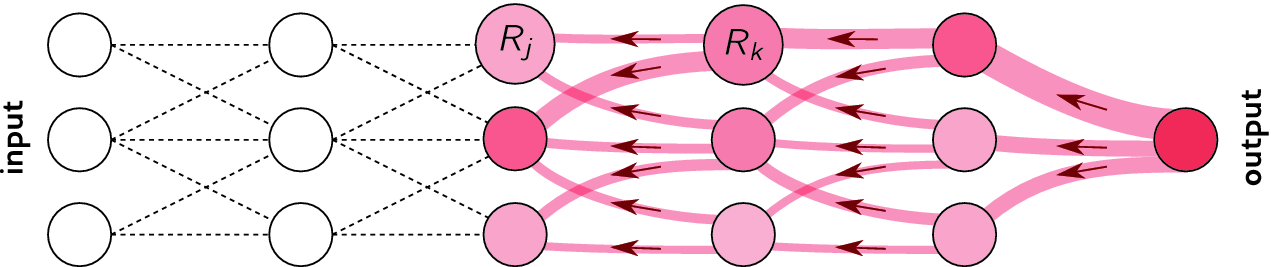
Illustration of the LRP procedure. Each neuron redistributes to the lower layer as much as it has received from the higher layer. ,Source : Springer
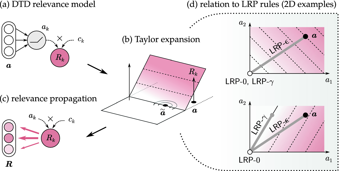
Illustration of DTD: (a) graph view of the relevance model, (b) function view of the relevance model and reference point at which the Taylor expansion is performed,(c) propagation of first-order terms on the lower layer. Source : Springer
Layer-wise relevance propagation [LRP] is a mathematical method which helps to bring explainability to deep neural network by propagating the prediction backward in the network. The content of this post is largely based on this book chapter with some of the additional information gained through detailed study and some experiments.
To get a brief overview of what is going to explain , please find some time to play with this interactive demo (Thanks to the makers ) and it is highly recommended to watch this before going in details to rest of the post. The major benefit of LRP is we don’t have to associate it with the network during training time , so the technique can be well applied to the already trained models.
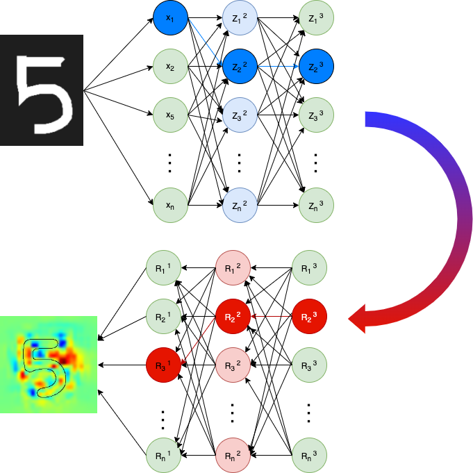
LRP operates by propagating the prediction f(x) backwards in the neural network. This concept is explained with little more clarity in the next section by considering the example of MNIST classification using CNN based approach.
High Level summary on working of LRP
This image show a big picture on how the forward pass happens and how the relevance score is built and visualise it using heat-map
“LRP Works on the principle of conservation . We have the output layer , back propagation process and the input layer.Magnitude of any output neuron is conserved through the back-propagation process and this value will be equal to the sum of the relevance map of the input layer.”
With the property in the left side, we can explain LRP in a simple way. In the output layer, we have to identify one neuron which needs explanation. Assign the relevance of picked neuron as the activation value and assign the relevance of other neurons in the output layer to zero.
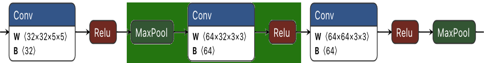
In the above picture, the input to the Conv layer is the output of MaxPool layer and output of Conv layer is connected to the input of Relu activation. Now if we want to identify the relevance score of Conv , select one neuron from the input of Relu , keep all other input as zero and find how the network arrived at selected neuron value.
Step by Step understanding on working of Layer-Wise Relevance Propagation
We mentioned about how to pick a neuron from the output layer and keep the relevance score same as activation in the previous section. Once the above step is completed , the next step is to go backward through the network. We use the basic LRP rule here (LRP-0)
R_j = \sum _k \frac{a_j w_{jk}}{\sum _{0,j} a_j w_{jk}} R_kHere
j,k is 2 neurons of the consecutive layer
R is relevance score of previous layer ( in this case it is activation value which we choose )
a is activation of current neuron
w is the weight between current and previous neuron.
What we applied here is the simple rule of LRP. Depends on the type of neurons , there are various LRP rules which we can use to bring the clear explanation. These rules are detailed in next section.
Implementation of LRP for Dense Layer
def r_dense(self, a, w, r):
        # relevance propagation rules for dense layers.
        # Args:
        #    a: activations
        #    w: weights
        #    r: relevance scores
        # Returns: relevance scores
        weight_pos = tf.maximum(w, 0.0)
        z = tf.matmul(x, weight_pos) + self.epsilon
        s = r / z
        c = tf.matmul(s, tf.transpose(weight_pos))
        return c * x
LRP as a Deep Taylor Decomposition [DTD]
Before going into details of rules, we will discuss a little on relationship between LRP and Deep Taylor Decomposition . This relation has been introduced in the Deep Taylor Decomposition paper by the authors of LRP. DTD views LRP as a succession of Taylor expansions performed locally at each neuron. This paper introduce a decomposition method based on the Taylor expansion of the function at some well-chosen root point.A root point is a point where
f(x˜)=0
The first-order Taylor expansion of f(x) is given by
f(x)=f(x˜)+(∂f∂x∣x=x˜)⊤⋅(x-x˜)+ε=0+∑p∂f∂xp∣x=x˜⋅(xp-x˜p)︸Rp(x)+ε,
First-order terms (summed elements) identify how much of Rk should be redistributed on neurons of the lower layer. Due to the potentially complex relation
between a and Rk, finding an appropriate reference point and computing the gradient locally is difficult.
LRP Rules
Detailed LRP Rules on left side with little more expiation to main rules.
In a nutshell, LRP uses the weights and the activations created by the forward-pass to propagate the output back through the network up until the input layer. There, we can visualize which pixels really contributed to the output.
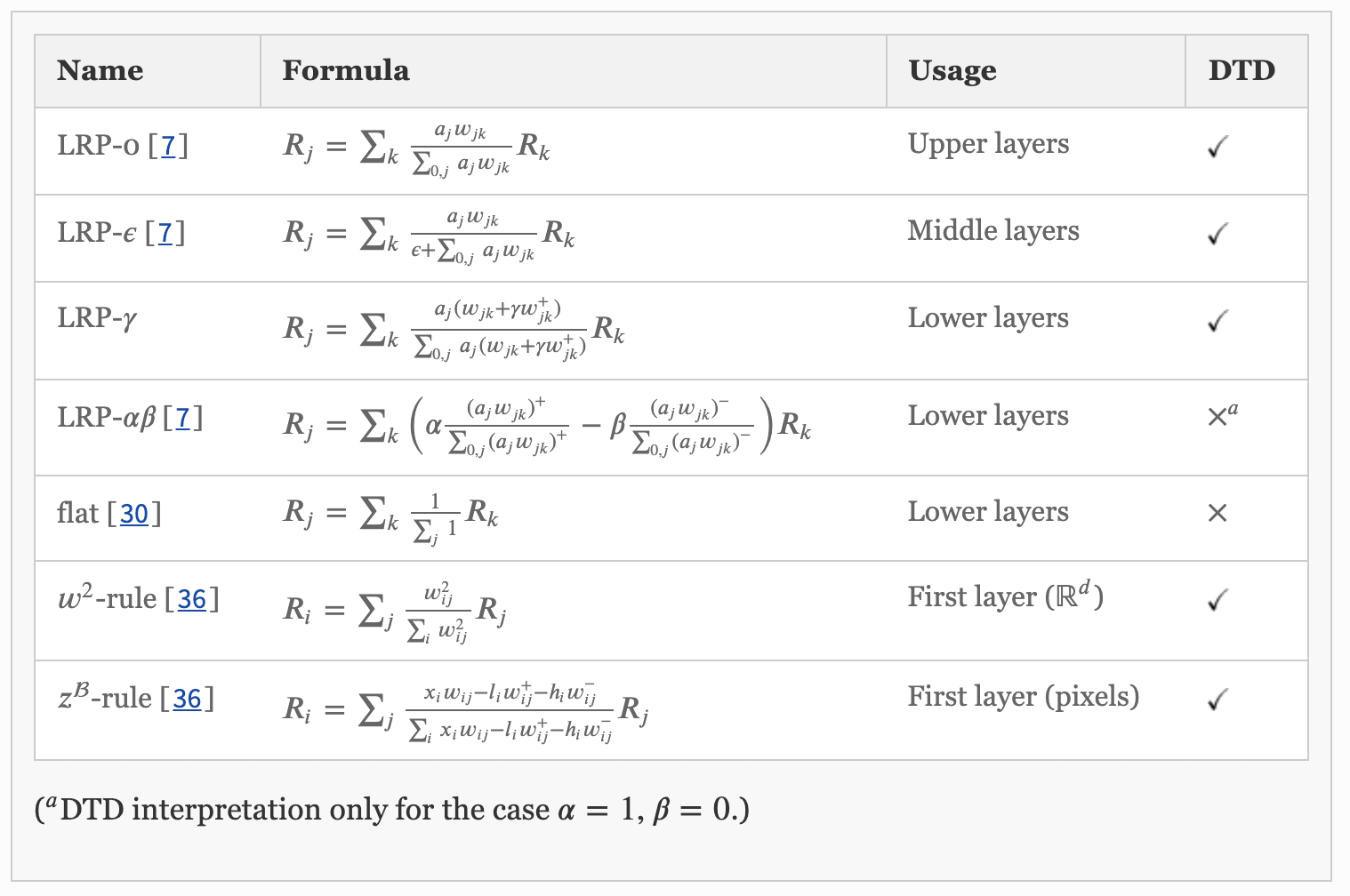
Source : Springer
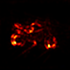
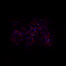
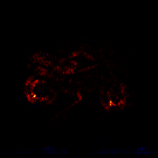
The image was classified as moped with a classification score of 16.63 and the true class is motor scooter. We can observe the kind of heat-map produced by different rule of LRP.
LRP Rules & Generated Heat-maps

Input image

LRP Alpba-Beta
LRP_Composite flat

LRP-Composite
LRP-Epsilon
LRP Alpha-Beta +W2
Heat-maps generated by LRP are very helpful to understand and visualize what the algorithm has learned.
Major contribution of LRP in NN Explainability is as follows.
Localisation: Pinpoint the exact location of action in the input.
Feature ranking: Calculates the contribution of each features to the final output.
Visualisation: Provide visualisation to understand how the algorithm is learning.
Input Layer
These layers are different from intermediate layers as there is no activations comes as input instead , we get pixels or real values. So zB-rule is good for pixels and w2 rule is good for other values.
R_i = \sum _j \frac{x_i w_{ij} - l_i w_{ij}^+ - h_i w_{ij}^- }{\sum _{i} x_i w_{ij} - l_i w_{ij}^+ - h_i w_{ij}^-} R_jHigher Layers
Here the propagation rule will be close to the function and its gradient. LRP-0 picks many local artefacts. The explanation generated will be complex and neither faithful nor understandable.
R_j = \sum _k \frac{a_j w_{jk}}{\sum _{0,j} a_j w_{jk}} R_kMiddle Layers
Middle layers are often stacked and involves weight sharing. This introduces spurious variations. LRP-ϵ helps to filter out spurious variations and maintains only important explanation factors.LRP-ϵ removes all noise elements from the explanation.
R_j = \sum _k \frac{a_j w_{jk}}{\epsilon + \sum _{0,j} a_j w_{jk}} R_kLower layers
As we approach the lower layers , we want the explanation to be more smoother with less noise elements. Here most working rule is LRP-γ because of its property of favouring positive evidence over negative evidence . Because of this property , LRP-γ makes the features more densely highlighted which makes it more human understandable form. Here one thing to carefully handled is , it can highlight some unimportant objects in the scene.
R_j = \sum _k \frac{a_j (w_{jk} + \gamma w_{jk}^+)}{\sum _{0,j} a_j (w_{jk} + \gamma w_{jk}^+)} R_kOutput layers
LRP-0 is the best rule in output layers to the propagation to be more close to the function.
R_j = \sum _k \frac{a_j w_{jk}}{\sum _{0,j} a_j w_{jk}} R_kConclusion
References
[1] Grégoire MontavonAlexander BinderSebastian LapuschkinWojciech SamekKlaus-Robert Müller, et al. ” Layer-Wise Relevance Propagation: An Overview” 978-3-030-28954-6_10
[2] Woo-Jeoung Nam, Shir Gur, Jaesik Choi, Lior Wolf,, Seong-Whan Lee, et al. “Relative Attributing Propagation: Interpreting the Comparative Contributions of Individual Units in Deep Neural Networks“, arXiv:1904.00605v4 [cs.CV] 13 Nov 2019
[3] Vignesh Srinivasan; Sebastian Lapuschkin; Cornelius Hellge; Klaus-Robert Müller; Wojciech Samek, et ai, Interpretable human action recognition in compressed domain
[4] GrégoireMontavon SebastianLapuschkin AlexanderBinder WojciechSamek Klaus-RobertMüller ,et aI, Explaining nonlinear classification decisions with deep Taylor decomposition
[5] Eugen Lindwurm, et al. InDepth: Layer-Wise Relevance Propagation
[6] Jianming Zhang, Zhe Lin, Jonathan Brandt, Xiaohui Shen, Stan Sclaroff1 ,et aI , “Top-down Neural Attention by Excitation Backprop” arXiv:1608.00507v1 [cs.CV] 1 Aug 2016.